Classification in Data Mining

Introduction

Classification constructs the classification model by using training data set.
Classification predicts the value of classifying attribute or class label.
For example: Classification of credit approval on the basis of customer data.
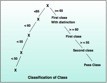
University gives class to the students based on marks.
If x >= 65, then First class with distinction.
If 60<= x<= 65, then First class.
If 55<= x<=60, then Second class.
If 50<= x<= 55, then Pass class.

Classification Requirements

The two important steps of classification are:

1. Model construction

A predefine class label is assigned to every sample tuple or object. These tuples or subset data are known as training data set.
The constructed model, which is based on training set is represented as classification rules, decision trees or mathematical formulae.

2. Model usage

The constructed model is used to perform classification of unknown objects.
A class label of test sample is compared with the resultant class label.
Accuracy of model is compared by calculating the percentage of test set samples, that are correctly classified by the constructed model.
Test sample data and training data sample are always different.

Classification vs Prediction

Classification	Prediction
It uses the prediction to predict the class labels.	It is used to assess the values of an attribute of a given sample.
For example: If the patients are grouped on the basis of their known medical data and treatment outcome, then it is considered as classification.	For example: If a classification model is used to predict the treatment outcome for a new patient, then it is prediction.

Issues related to Classification and Prediction

1. Data preparation
Data preparation consist of data cleaning, relevance analysis and
data transformation.

2. Evaluation of classification methods
i) Predictive accuracy: This is an ability of a model to predict the class label of a new
or previously unseen data.
ii) Speed and scalability: It refers to the time required to construct and use the model and increase efficiency in disk- resident databases.

3. Inter-predictability:
It is an understanding and insight provided by the model.

Decision Tree Induction Method

Decision tree:

A decision tree performs the classification in the form of tree structure. It breaks down the dataset into small subsets and a decision tree can be designed simultaneously.
The final result is a tree with decision node.

For example:
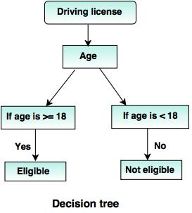
The following decision tree can be designed to declare a result, whether an applicant is eligible or not eligible to get the driving license.

Attribute selection methods

1. Gini Index (IBM intelligent Miner)

Gini index is used in CART (Classification and Regression Trees), IBM's Intelligent Miner system, SPRINT (Scalable Parallelizable Induction of decision Trees).
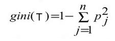
If a data set 'T' contains examples from 'n' classes, gini index, gini (T) is defined as:

After splitting T into two subsets T₁, T₂ with sizes N₁ and N₂, the gini index of the split data is defined as:
gini_split (T) = N₁/ N₂ gini (T₁) + N₂/ N gini (T₂)
For each attribute, each of the possible binary splits is considered. For each attribute, the attribute providing smallest gini_split (T) is chosen to split the node for continuous- valued attributes, where each possible split-point must be considered.

2. ID3 (Algorithm for inducing a decision Tree)

Ross Quinlin developed ID3 algorithm in 1980.
C4.5 is an extension of ID3.
It avoids over-fitting of the data.
It determines the depth of decision tree and reduces the error pruning.
It also handles continuous value attributes. For example: salary or temperature.
It works for missing value attribute and handles suitable attribute selection measure.
It gives better efficiency of computation.

Algorithm to generate a decision tree from the training tuples of data partition, D.
Step 1: Create a node 'N':
Step 2: If tuple in D are all of the same class, 'C', then go to step 3
Step 3: Return 'N' as a leaf node labeled with the majority class in 'C'
Step 4: If attribute list is empty, then return 'N' as a leaf node labeled with the majority class in D.
Step 5: Apply attribute_selection_method (D, attribute _list) to find the “best” splitting criteria.
Step 6: If splitting_attribute is discrete-valued and multi way, splits are allowed. Then follow step 7
Step 7: Attribute_list ← attribute_list – splitting_attribute;// remove splitting attribute.
Step 8: For each outcome j of splitting creation, Let D_j be the set of data tuples in D that satisfies outcome j, If D_j is empty, then attached leaf is labeled with the majority class in D to node N;
Step 9: Else, attach the node returned by Generate_decision_tree (D_j, attribute_list ) to node N;
Step 10: Return N;
Step 11: Stop.

3. Tree Pruning

To avoid the overfitting problem, it is necessary to prune the tree.
Generally, there are two possibilities while constructing a decision tree. Some record may contain noisy data, which increases the size of the decision tree. Another possibility is, if the number of training examples are too small to produce a representative sample of the true target function.
Pruning can be possible in a top down or bottom up fashion.

Some well known methods to perform pruning are:

1. Reduced error pruning
This is simplest method of pruning. Start from the leaves. Each node is replaced with its most popular class to maintain accuracy.

2. Cost complexity pruning

It generates a series of trees.
Consider 'T₀' as the initial tree and 'T_m' as root.
Consider that the tree is created by removing a subtree from tree i- 1 and replacing it with a leaf node with value chosen as per the tree constructing algorithm.
The subtree which is removed can be chosen as follows:
Define the error rate of tree 'T' over data set 'S' as err (T,S).
The subtree from tree that minimizes is chosen for removal.
The function (T,t) defines the tree, which is obtained by pruning the subtrees 't' from the tree 'T'. After creating series of tree, the best tree is chosen by measuring a training set or cross-validation.

3. Alpha-beta pruning

It is a search algorithm, which improves the minimax algorithm by eliminating branches which will not be able to give further outcome.
Let alpha (α) be the value of the best choice along the path for higher value as MAX.
Let beta (β) be the value of the best choice along the path for lower value as MIN.
While working with decision tree, the problem of missing values (those values which are missing or wrong) may occur.
So, one of the most common solution is to label that missing value as blank.

Prediction

Prediction deals with some variables or fields, which are available in the data set to predict unknown values regarding other variables of interest.
Numeric prediction is the type of predicting continuous or ordered values for given input.
For example: The company may wish to predict the potential sales of a new product given with its price.
The most widely used approach for numeric prediction is regression.