Regression involves predictor variable (the values which are known) and response variable (values to be predicted).
The two basic types of regression are: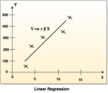
Solution:
Required formula:
P (c | x) = P (c | x) P (c) / P (x) In the fields of science, engineering and statistics, the accuracy of a measurement system is the degree of closeness of measurements of a quantity to that quantity's true value.
Where,
P (c | x) is the posterior of probability.
P (c) is the prior probability.
P (c | x) is the likelihood.
P (x) is the prior probability.
It is necessary to classify a <Blue, Indian, Sports>, is unseen sample, which is not given in the data set.
So the probability can be computed as:
P (Yes) = 5/10
P (No) = 5/10
So, unseen example X = <Blue, Indian, Sports>
P(X|Yes). P(Yes) = P(Blue|Yes). P(Indian|Yes). P(Sports|Yes). P(Yes)
= 3/5*2/5*1/5*5/10 = 0.024
P(X|No). P(No) = P(Blue|No). P(Indian|No). P(Sports|No).P(No)
= 2/5*3/5*3/5*5/10 = 0.072
So, 0.072 > 0.024 so example can be classified as NO.
The two basic types of regression are:
1. Linear regression
- It is simplest form of regression. Linear regression attempts to model the relationship between two variables by fitting a linear equation to observe the data.
- Linear regression attempts to find the mathematical relationship between variables.
- If outcome is straight line then it is considered as linear model and if it is curved line, then it is a non linear model.
- The relationship between dependent variable is given by straight line and it has only one independent variable.
Y = α + Β X - Model 'Y', is a linear function of 'X'.
- The value of 'Y' increases or decreases in linear manner according to which the value of 'X' also changes.
2. Multiple regression model
- Multiple linear regression is an extension of linear regression analysis.
- It uses two or more independent variables to predict an outcome and a single continuous dependent variable.
Y = a0 + a1 X1 + a2 X2 +.........+ak Xk +e
where,
'Y' is the response variable.
X1 + X2 + Xk are the independent predictors.
'e' is random error.
a0, a1, a2, ak are the regression coefficients.
Naive Bays Classification Solved example
Bike Damaged example: In the following table attributes are given such as color, type, origin and subject can be yes or no.| Bike No | Color | Type | Origin | Damaged? |
|---|---|---|---|---|
| 10 | Blue | Moped | Indian | Yes |
| 20 | Blue | Moped | Indian | No |
| 30 | Blue | Moped | Indian | Yes |
| 40 | Red | Moped | Indian | No |
| 50 | Red | Moped | Japanese | Yes |
| 60 | Red | Sports | Japanese | No |
| 70 | Red | Sports | Japanese | Yes |
| 80 | Red | Sports | Indian | No |
| 90 | Blue | Sports | Japanese | No |
| 100 | Blue | Moped | Japanese | Yes |
Solution:
Required formula:
P (c | x) = P (c | x) P (c) / P (x) In the fields of science, engineering and statistics, the accuracy of a measurement system is the degree of closeness of measurements of a quantity to that quantity's true value.
Where,
P (c | x) is the posterior of probability.
P (c) is the prior probability.
P (c | x) is the likelihood.
P (x) is the prior probability.
It is necessary to classify a <Blue, Indian, Sports>, is unseen sample, which is not given in the data set.
So the probability can be computed as:
P (Yes) = 5/10
P (No) = 5/10
| Color | |
| P(Blue|Yes) = 3/5 | P(Blue|No) = 2/5 |
| P(Red|Yes) = 2/5 | P(Red|No) = 3/5 |
| Type | |
| P(Sports|Yes) = 1/5 | P(Sports|No) = 3/5 |
| P(Moped|Yes) = 4/5 | P(Moped|No) = 2/5 |
| Origin | |
| P(Indian|Yes) = 2/5 | P(Indian|No) = 3/5 |
| P(Japanese|Yes) = 3/5 | P(Japanese|No) = 2/5 |
So, unseen example X = <Blue, Indian, Sports>
P(X|Yes). P(Yes) = P(Blue|Yes). P(Indian|Yes). P(Sports|Yes). P(Yes)
= 3/5*2/5*1/5*5/10 = 0.024
P(X|No). P(No) = P(Blue|No). P(Indian|No). P(Sports|No).P(No)
= 2/5*3/5*3/5*5/10 = 0.072
So, 0.072 > 0.024 so example can be classified as NO.